
Discrete Non-Contractual
For discrete, noncontractual business settings
import numpy as np
import pandas as pd
from scipy.optimize import minimize
import scipy.special as sc
import os
from IPython.display import display, Image
import plotly.graph_objs as go
import pprint
def shape(df):
    '''TODO: Shapes transactional data into recency and frequency'''
    pass

def i_likelihood(alpha, beta, gamma, delta, x, t_x, n):
    '''Calculates the individual likelihood for a person
    given paramters, frequency, recency, and periods
    '''
    # Summation component
    summation = [sc.beta(alpha+x, beta+t_x-x+i) / sc.beta(alpha, beta)
                 * sc.beta(gamma+1, delta+t_x+i) / sc.beta(gamma, delta)
                 for i in range(0, n-t_x)]

    # First component
    return (sc.beta(alpha+x, beta+n-x) / sc.beta(alpha, beta)
            * sc.beta(gamma, delta+n) / sc.beta(gamma, delta)
            + sum(summation))

def log_likelihood(df, alpha, beta, gamma, delta):
    '''Computes total log-likelihood for given parameters'''
    # Get frequency, recency, and periods lists
    frequency = df.frequency.to_list()
    recency = df.recency.to_list()
    periods = df.periods.to_list()

    # Compute individual likelihood first
    indiv_llist = [i_likelihood(alpha, beta, gamma, delta, frequency[i], recency[i], periods[i])
                   for i in range(0, len(frequency))]

    # Multiply with num_obs
    num_obs = np.array(df.num_obs.to_list())

    return np.sum(num_obs * np.log(np.array(indiv_llist)))


def maximize(df):
    '''Maximize log-likelihood by searching for best
    (alpha, beta, gamma, delta) combination'''
    func = lambda x: -log_likelihood(df, x[0], x[1], x[2], x[3])
    x0 = np.array([1., 1., 1., 1.])
    res = minimize(func, x0, method='Nelder-Mead', options={'xtol': 1e-8, 'disp': False})
    return res.x


def prob_alive(df, x, t_x, p):
    '''Probability for a customer with transaction
    history (x, t_x, n) to be alive at time period p'''
    alpha, beta, gamma, delta = maximize(df)
    n = df.periods.iloc[0]
    indiv_ll = i_likelihood(alpha, beta, gamma, delta, x, t_x, n)
    return (sc.beta(alpha+x, beta+n-x) / sc.beta(alpha, beta)
            * sc.beta(gamma, delta+p) / sc.beta(gamma, delta)
            / indiv_ll)

def prob_alive_df(df, p):
    '''List of probabilities for a customer to be alive
    for all the combinations of (x, t_x)'''
    alpha, beta, gamma, delta = maximize(df)
    n = df.periods.iloc[0]

    x_list = df.frequency.to_list()
    t_x_list = df.recency.to_list()

    p_list = [sc.beta(alpha+x_list[i], beta+n-x_list[i])
               / sc.beta(alpha, beta)
               * sc.beta(gamma, delta+p) / sc.beta(gamma, delta)
               / i_likelihood(alpha, beta, gamma, delta, x_list[i], t_x_list[i], n)
               for i in range(0, len(x_list))]

    return pd.DataFrame({'frequency': x_list,
                         'recency': t_x_list,
                         'p_alive': p_list})

def expected_count(df, n):
    '''Calculates the mean number of transactions
    occurring across the first n transaction opportunities
    '''
    alpha, beta, gamma, delta = maximize(df)
    E_x = [alpha / (alpha+beta)
           * delta / (gamma-1)
           * (1-sc.gamma(gamma+delta)/sc.gamma(gamma+delta+i)
           * sc.gamma(1+delta+i)/sc.gamma(1+delta))
           for i in range(1, n+1)]
    return pd.DataFrame({'n': np.arange(1, n+1),
                         'E[X(n)]': E_x,
                        })

def pmf(df, x, alpha, beta, gamma, delta):
    '''probabilility of having x transactions in the dataset
    (essentially the pmf)'''
    n = df.periods.iloc[0]

    # Summation component
    summation = [sc.comb(i, x)
                 * sc.beta(alpha+x, beta+t_x-x+i) / sc.beta(alpha, beta)
                 * sc.beta(gamma+1, delta+t_x+i) / sc.beta(gamma, delta)
                 for i in range(0, n-t_x)]

    return (sc.comb(n, x)
            * sc.beta(alpha+x, beta+n-x) / sc.beta(alpha, beta)
            * sc.beta(gamma, delta+n) / sc.beta(gamma, delta)
            + sum(summation))


def pmf_df(df):
    '''
    Creates a dataframe for all possible x's
    '''
    alpha, beta, gamma, delta = maximize(df)
    p_x = [pmf(df, i, alpha, beta, gamma, delta)
           for i in range(0, df.periods.loc[0]+1)]

    return pd.DataFrame({'x': np.arange(0, df.periods.loc[0]+1),
                         'p': p_x})


def cond_expectations(alpha, beta, gamma, delta, x, t_x, n, p):
    '''The expected number of future transactions
    across the next p transaction opportunities by
    a customer with purchase history (x, t_x, n)'''
    return (1/i_likelihood(alpha, beta, gamma, delta, x, t_x, n)
            * sc.beta(alpha+x+1, beta+n-x)/sc.beta(alpha, beta)
            * delta/(gamma-1)
            * sc.gamma(gamma+delta)/sc.gamma(1+delta)
            * (sc.gamma(1+delta+n)/sc.gamma(gamma+delta+n)
             - sc.gamma(1+delta+n+p)/sc.gamma(gamma+delta+n+p))
           )


def cond_expectations_df(df, p):
    '''Creates a dataframe for CE for each
    (x, t_x, n) combination'''
    alpha, beta, gamma, delta = maximize(df)
    x_list = df.frequency.to_list()
    t_x_list = df.recency.to_list()
    n_list = df.periods.to_list()

    ce_list = [cond_expectations(alpha, beta, gamma, delta,
                                 x_list[i], t_x_list[i], n_list[i], p)
               for i in range(0, len(x_list))]

    return pd.DataFrame({'frequency': x_list,
                         'recency': t_x_list,
                         'n': n_list,
                         'ce': ce_list})


def marg_posterior_p(alpha, beta, gamma, delta, x, t_x, n, p):
    '''The marginal posterior distribution of p'''
    b1 = (p**(alpha+x-1) * (1-p)**(beta+n-x-1)
         / sc.beta(alpha, beta)
         * sc.beta(gamma, delta+n)/sc.beta(gamma, delta))
    b2 = [(p**(alpha+x-1) * (1-p)**(beta+t_x-x+i-1)
          / sc.beta(alpha, beta)
          * sc.beta(gamma+1, delta+t_x+i)
          / sc.beta(gamma, delta))
          for i in range(0, n-t_x)]
    return (b1 + sum(b2)) / ilikelihood(alpha, beta, gamma, delta, x, t_x, n)


def marg_posterior_theta(alpha, beta, gamma, delta, x, t_x, n, theta):
    '''The marginal posterior distribution of theta'''
    c1 = (sc.beta(alpha+x, beta+n-x) / sc.beta(alpha, beta)
          * theta**(gamma-1) * (1-theta)**(delta+n-1)
          / sc.beta(gamma, delta))
    c2 = [(sc.beta(alpha+x, beta+t_x-x+i) / sc.beta(alpha, beta)
          * theta**gamma * (1-theta)**(delta+t_x+i-1) / sc.beta(gamma, delta))
          for i in range(0, n-t_x)]
    return (c1 + sum(c2)) / ilikelihood(alpha, beta, gamma, delta, x, t_x, n)
df = pd.read_csv('../data/discrete-noncontractual.csv')
df.head()
alpha, beta, gamma, delta = maximize(df)
alpha, beta, gamma, delta
prob_alive_df(df, 6)
Matches with slide 76 of Lecture 7
expected_count(df, 11)
Matches E[X(n)] column in
BGBB_2011-01-20.csvfrom http://brucehardie.com/notes/010/
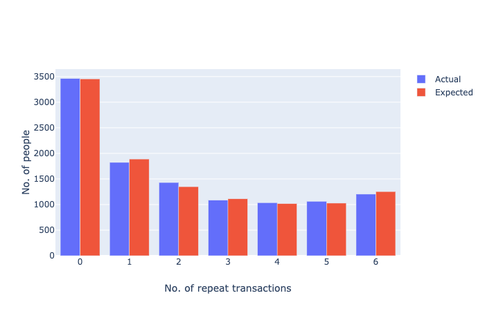
count_df = pd.read_csv('../data/discrete-noncontractual-3.csv')
count_df = (
    count_df
    .merge(pmf_df(df), on='x')
    .assign(
        Model=lambda x: x['p'] * 11104
    )
)
count_df
Matches up with P(X(n)=x) column in
BGBB_2011-01-20.csvfrom http://brucehardie.com/notes/010/
Image(filename='../images/discrete-noncontractual-figure-1.png')
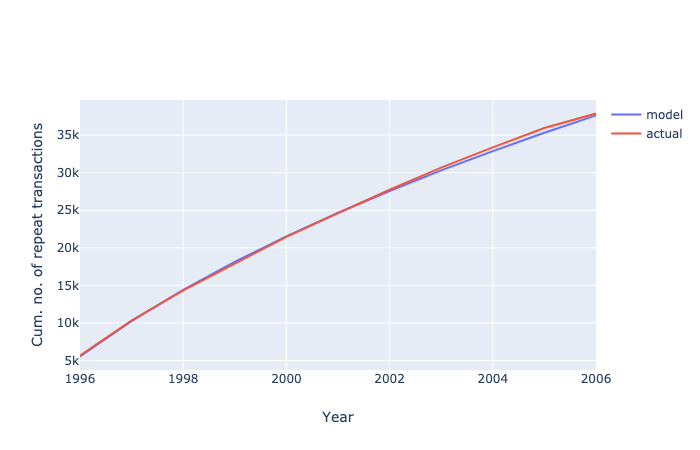
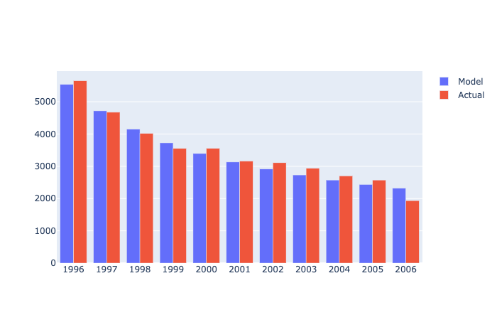
incr_df = pd.read_csv('../data/discrete-noncontractual-2.csv')
# Add a cumulative sum column
incr_df['cumulative'] = incr_df['Actual'].cumsum()
incr_df
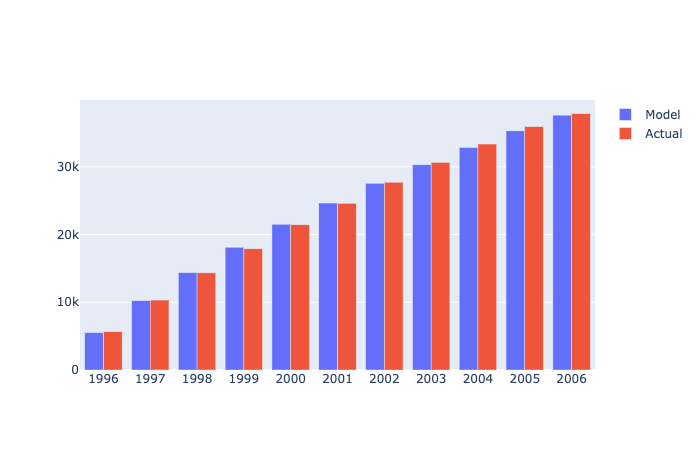
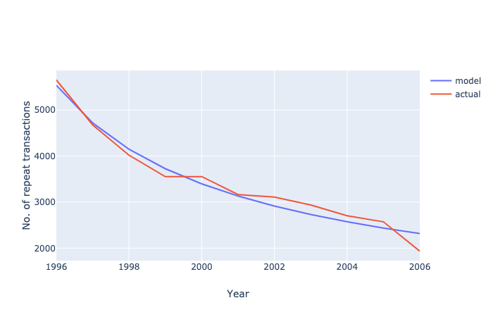
expected_df = (
    expected_count(df, 11)
    .assign(
        model=lambda x: x['E[X(n)]'] * 11104,
        Year=np.arange(1996, 2007),
        annual=lambda x: x['model'].diff()
    )
)
expected_df.loc[0, 'annual'] = expected_df['model'].iloc[0]
expected_df
Image('../images/discrete-noncontractual-figure-2.png')
Image('../images/discrete-noncontractual-figure-4.png')
Image('../images/discrete-noncontractual-figure-3.png')
Image('../images/discrete-noncontractual-figure-5.png')
ce_df = cond_expectations_df(df, 5)
ce_df
Matches up with CE column in
BGBB_2011-01-20.csvfrom http://brucehardie.com/notes/010/
ce_df.pivot_table(values='ce', index='frequency', columns='recency')
(
    ce_df
    .groupby('frequency', as_index=False)
    .agg(
        mean_ce=('ce', 'mean')
    )
)
(
    ce_df
    .groupby('recency', as_index=False)
    .agg(
        mean_ce=('ce', 'mean')
    )
)
# TODO
p_alive_df = prob_alive_df(df, 7)

p_alive_df.pivot_table(values='p_alive', index='frequency', columns='recency')
def post_dist(alpha, beta, gamma, delta, x, t_x, n, p, theta):
    '''Joint Posterior of p and theta
    actually i am not sure if this is right'''
    g_p = p**(alpha-1) * (1-p)**(beta-1) / sc.beta(alpha, beta)
    g_theta = theta**(gamma-1) * (1-theta)**(delta-1) / sc.beta(gamma, delta)
    l_p_theta_1 = (p**x) * (1-p)**(n-x) * (1-theta)**n
    l_p_theta_2 = [(p**x) * (1-p)**(t_x-x+i) * theta * (1-theta)**(t_x+i)
                   for i in range(0, n-t_x)]
    l_p_theta = l_p_theta_1 + sum(l_p_theta_2)
    l_abgd = i_likelihood(alpha, beta, gamma, delta, x, t_x, n)
    return l_p_theta * g_p * g_theta / l_abgd
def beta_distribution(p, alpha, beta):
    return p**(alpha-1) * (1-p)**(beta-1) / sc.beta(alpha, beta)
def expected_value(darray):
    '''Gets expected value of p in darray'''
    probs = np.array(darray) / np.sum(darray)
    sample = np.random.choice(np.arange(0.00, 1.00, 1.0 / len(darray)),
                              size=100000, replace=True, p=probs)
    return np.mean(sample)
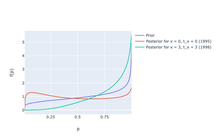
zerozero = [marg_posterior_p(alpha, beta, gamma, delta, 0, 0, 6, i) for i in np.arange(0.00, 1.00, 0.001)]
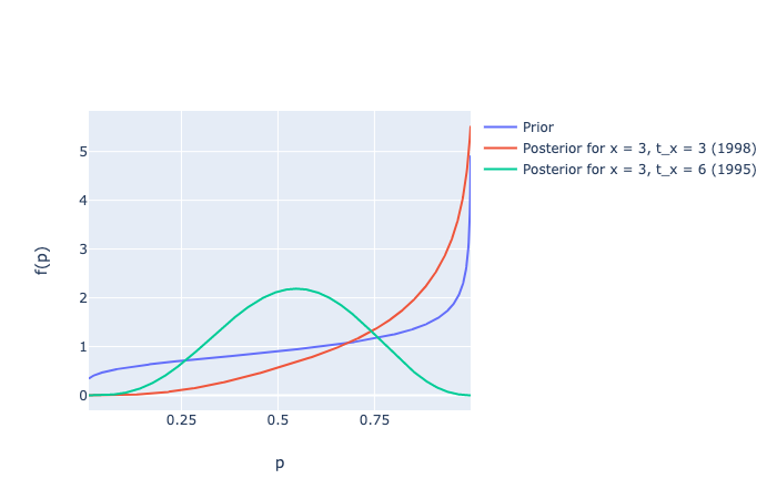
threethree = [marg_posterior_p(alpha, beta, gamma, delta, 3, 3, 6, i) for i in np.arange(0.00, 1.00, 0.001)]
threesix = [marg_posterior_p(alpha, beta, gamma, delta, 3, 6, 6, i) for i in np.arange(0.00, 1.00, 0.001)]
p_betas = [beta_distribution(i, alpha, beta) for i in np.arange(0.01, 1.00, 0.001)] # prior
# Slide 78 from Lecture 7
Image("../images/discrete-noncontractual-figure-6.png")
Image("../images/discrete-noncontractual-figure-7.png")
# Expected Values
pp = pprint.PrettyPrinter()
some_dict = {'prior': alpha / (alpha+beta),
             'x = 0, t_x = 0': expected_value(zerozero),
             'x = 3, t_x = 3': expected_value(threethree),
             'x = 3, t_x = 6': expected_value(threesix)}

pp.pprint(some_dict)
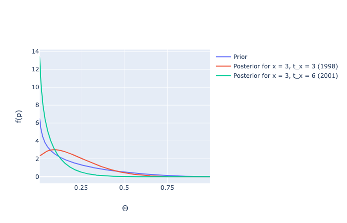
threethree_theta = [marg_posterior_theta(alpha, beta, gamma, delta, 3, 3, 6, i) for i in np.arange(0.01, 1.00, 0.001)]
threesix_theta = [marg_posterior_theta(alpha, beta, gamma, delta, 3, 6, 6, i) for i in np.arange(0.01, 1.00, 0.001)]
theta_betas = [beta_distribution(i, gamma, delta) for i in np.arange(0.01, 1.00, 0.001)] # prior
Image('../images/discrete-noncontractual-figure-8.png')
# Expected Values
pp = pprint.PrettyPrinter()
some_dict = {'prior': gamma / (gamma+delta),
             'x = 3, t_x = 3': expected_value(threethree_theta),
             'x = 3, t_x = 6': expected_value(threesix_theta)}

pp.pprint(some_dict)
# TODO